As Brian Miller and Cornelius Hunter have already noted, an extraordinary scientific paper has just been published by Winston Ewert. Writing in the journal BIO-Complexity, Ewert proposes that life is best explained not by Darwin’s hypothesis of an ancestry tree, but by a modern design-inspired hypothesis of a dependency graph. The dependency graph model has been explained here. The original paper is here. 

I want to explain the math and the philosophy that allow us to objectively determine which model has the superior explanatory power.

From Simplicity to Probability

We want to choose the model that explains the data most simply. 

What is simplicity? It is the absence of complexity, the absence of parts, or the absence of options. Another way of looking at it is that there are many more ways to make a complex model than a simple model. Therefore, one way to measure the complexity of a model is to count how many ways there are to build a model like it. Then, assuming we don’t know the details of how natural processes would generate the particular pattern (or how an intelligent agent would choose it), we assume that each particular pattern is equally likely to be generated (or chosen). In other words, the probability of any particular model is the inverse of the number of models like it. In general, simple models are fewer in number, and simple models are intuitively considered to be more probable. On the other hand, complex models are much greater in number, and therefore considered to be less probable. Yet another way of looking at it is that complexity is a cost that we want to avoid: simple models are parsimonious. 

This correspondence between complexity and improbability is very useful, and we can use the two concepts interchangeably to help organize our thinking. What if you have a bunch of complex but similar models that each explain the data quite well? Then you group them together into a more probable model, which is a bit like coarse graining a model into a simpler model with fewer specific elements.

In Bayesian Model Selection, the best model is the one that makes the data most probable. There is no point in having a simple model if it does not explain the data (if the probability of the data is zero). Likewise there is no point in having a model that is more complex (and thus even less improbable) than the data it needs to explain. That would be overfitting. The overall complexity is the probability of the model combined with the probability of the data given the model. In Ewert’s paper, there are two overarching models that we want to distinguish: the ancestry tree, and the dependency graph, but there are myriad possible sub-models, each contributing to the overall probability of the overarching model. 

Average Values and Bayesian Priors

Unfortunately, both models (the tree of life and the dependency graph) are extremely complex, with a very large number of adjustable parameters. This might seem to make the question undecidable: We often argue that the tree of life is a terrible fit to the data, requiring numerous ad-hoc “epicycles” to make the data fit. We might further argue that a particular dependency graph is a better fit to the data. But a believer in common descent might reasonably respond that our theory is also not parsimonious; if you add enough modules you could explain literally anything, even random data. It seems that deciding between the two models can never be a rational decision; it seems it will always involve a good deal of intuition or even faith. Fortunately, however, there are ways to tame the complexity enough to get objective and meaningful answers.

The main strategy for coping with the complexity is summation (or mathematical integration) over all possibilities. Ewert handles many of the parameters by integration: these include the edge probability b (the expected connectivity) of the nodes and the different propensities to add α or lose λ  genes on each of the n nodes. This may seem strange, but it is standard probabilistic reasoning. If the probability distribution of Y (for example, the actual number of gene-losses) depends on X (for example, λ), but you don’t know X, you can still calculate the probability of Y if you have the probability distribution of X. In many cases we don’t even know what the true distribution of X would be. In such cases, Ewert assumes that every possibility has an equal probability (a flat distribution) because this should introduce the least bias. This may also seem strange, but it is quite common in Bayesian reasoning, where it is called a flat prior. Although the prior distribution of X is technically a choice, and yes that choice has some influence on the result, the way Bayesian reasoning works is that the more data you add, the less the particular choice of prior matters. The important thing is to choose a prior that is not biased; a prior that allows the data to speak, if you like. Bayesian reasoning is important in that it gives us some hope of escaping from the tyranny of fundamentalist presuppositions, whether evolutionist/naturalistic fundamentalism or creationist/biblical fundamentalism (though interestingly Thomas Bayes was a clergyman). 

The idea is that we want to make sure that the many things we don’t know don’t stop us from making reasonable inferences using what we do know. 

Calculating Bounds

Although some of the variables can be integrated mathematically, others cannot. This is a problem for both models since (in theory) we should sum all the probabilities from all possible assignments of genes to nodes and deletions from nodes. But it is a particular problem for the dependency graph: there are different possible numbers of nodes in the dependency graph, and myriad possible ways of connecting each number of nodes. To get a precise probability for the overarching dependency graph model, we would need to sum over every single one of these possible configurations. In practice these sums are impossible to do; there are far too many. 

However, even when it is not possible to calculate a precise probability, it is often possible to calculate bounds. This is a time-honored way of proving things without doing hard calculations, especially in mathematics. 

What is the probability of a teapot coalescing from atoms in orbit around the sun? Nobody knows. But, for example, you could say it is at least as improbable as a 100g collection of atoms overcoming thermodynamic entropy to stick together. This is an upper bound on the probability, and it is something that you could calculate quite easily (and, as it turns out, it is extremely improbable; effectively impossible).

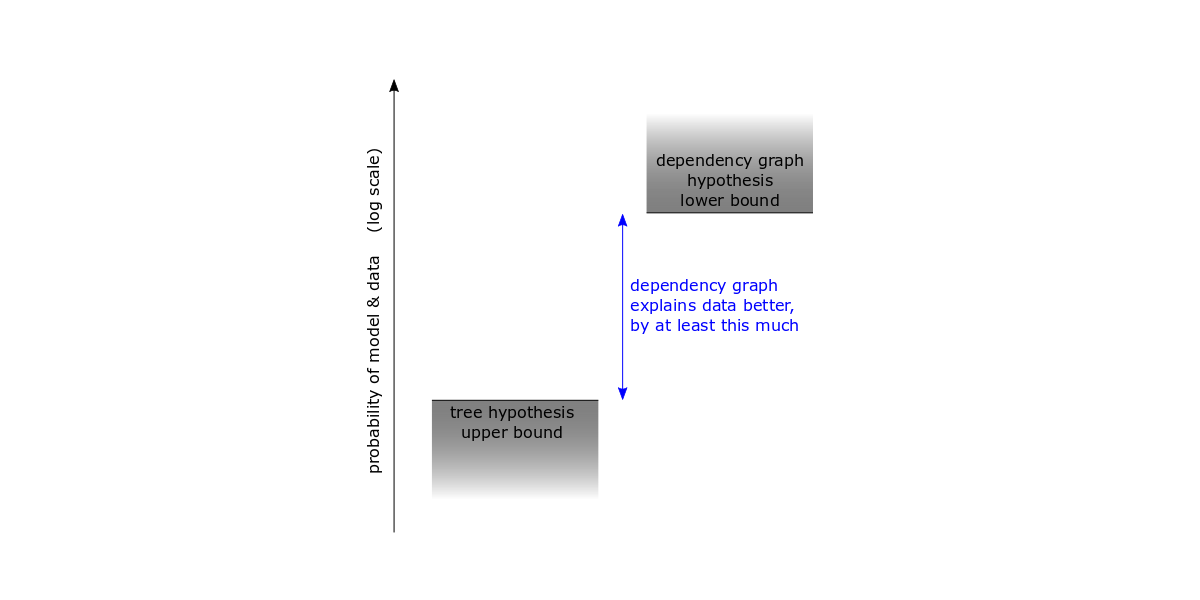
In order to show that the dependency graph is a better explanation, Ewert estimates an upper bound on the probability of the data given the ancestral tree hypothesis, and calculates a lower bound on the probability of the data given the dependency graph hypothesis, and then looks at the difference. 

Complexity of the Graph

The tree model has a big advantage in that it is simpler than the dependency graph model. If there are S species, then the tree model has (S-1) ancestral species. In contrast the dependency graph can have up to N_max = (2^S-1-s) optional modules. As S gets larger, this difference grows exponentially. For example, where there are 4 species (as in the figures below), there are up to 3 ancestral species, but up to 11 modules. Where there are just 10 species, there are 9 ancestral species, but up to 1013 possible modules! That is a lot of extra complexity.

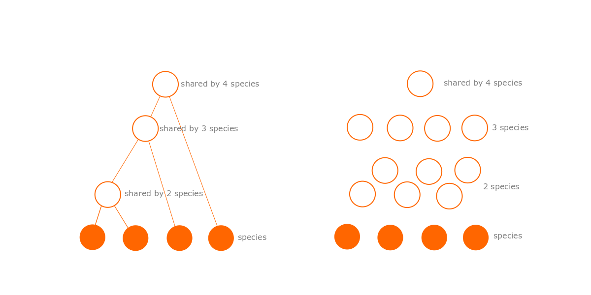
Secondly, the connections add complexity. A tree of N nodes has exactly (N-1) connections, but a graph of N nodes can have anyhere up to N(N-1)/2 possible connections. Each of these connections might exist or might not, giving a very large number of possibilities.  The probability of any particular combination of connections is very small, which translates into a very small probability for any particular graph.

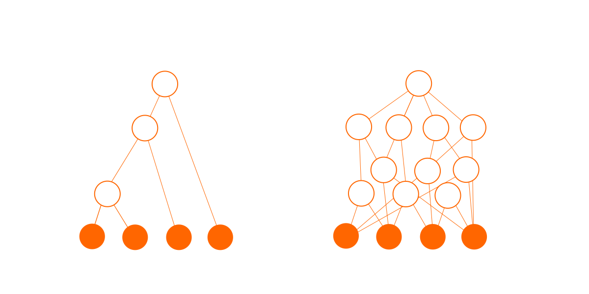
This dependency graph is not a real one; it is just my artistic impression to show the potential increase in complexity.

For the tree model, Ewert assumes that biologists have done a good job under the constraints of their model and found a good quality fit already, so he takes the hypothetical ancestral tree developed by expert biologists found at NCBI. Because we are calculating bounds, not precise probabilities, and because the tree is so much simpler, the calculation can be simplified by giving the tree a conditional probability of 1 (in words: if the tree hypothesis is true, then this tree is the correct tree). In contrast, every dependency graph is treated as highly improbable; there is a hefty penalty just for being a dependency graph. 

If all else were equal it would be far more parsimonious to choose the tree over the dependency graph. So why would anyone opt for the dependency graph? It’s because of the data. 

Complexity of the Data Given the Graph

The two models are given the same data to explain. The data Ewert chose was the distribution of gene families in species. These gene families were also taken from categories and data created by expert biologists, found in nine different public databases. 

Ewert’s algorithm then assigns these gene families to ancestral species on the tree, or modules on the dependency graph, to optimize the probability of each. Ewert follows the assumption of Dollo Parsimony, which means that each gene family appears only once in the history of life, or in no more than one designed module. 

The algorithm initially assigns each gene family to the purported common ancestor (according to the tree hypothesis) and then tries to improve on that. The tree and these gene assignments are also used as a first guess for the dependency graph. By default, nodes get all the genes from higher nodes they are connected to. In the case of the tree this means descendant species inherit genes from ancestral species. In the case of the dependency graph, this means modules import genes from their dependencies. To make the graph fit, some genes may need to be deleted once or many times from lower nodes. 

Ewert assumes that there is a certain probability of adding a gene to each node, but since we don’t know what it is, he averages over all possible probabilities. The formula is also given in equation 4 of the paper. He also assumes that gene deletions happen with a certain probability in each node, but since we don’t know what that probability is, he averages over all possible probabilities. The formula is also given in equation 6 of the paper. The effect is that the first addition/deletion costs a penalty that depends on the number of genes, and then subsequent additions/deletions cost slightly less and so on. The consequence is that it may be more probable to add a gene higher up the tree/graph or delete it further down the graph, even if that means deleting it more times. So there is also an algorithm that tries to move gene-family assignments up the tree or graph, and/or deletions down the tree or graph, if that would give a better probability. In the case of the dependency graphs, the algorithm also creates or removes entire modules where that would give better probabilities. This last algorithm is what allows the discovery of dependency graphs that are radically different from a tree. 

Consider these two imaginary sets of data. Each row or color is a gene family, and each column is a species. A filled circle indicates that that species has a representative of that gene family in its genome.

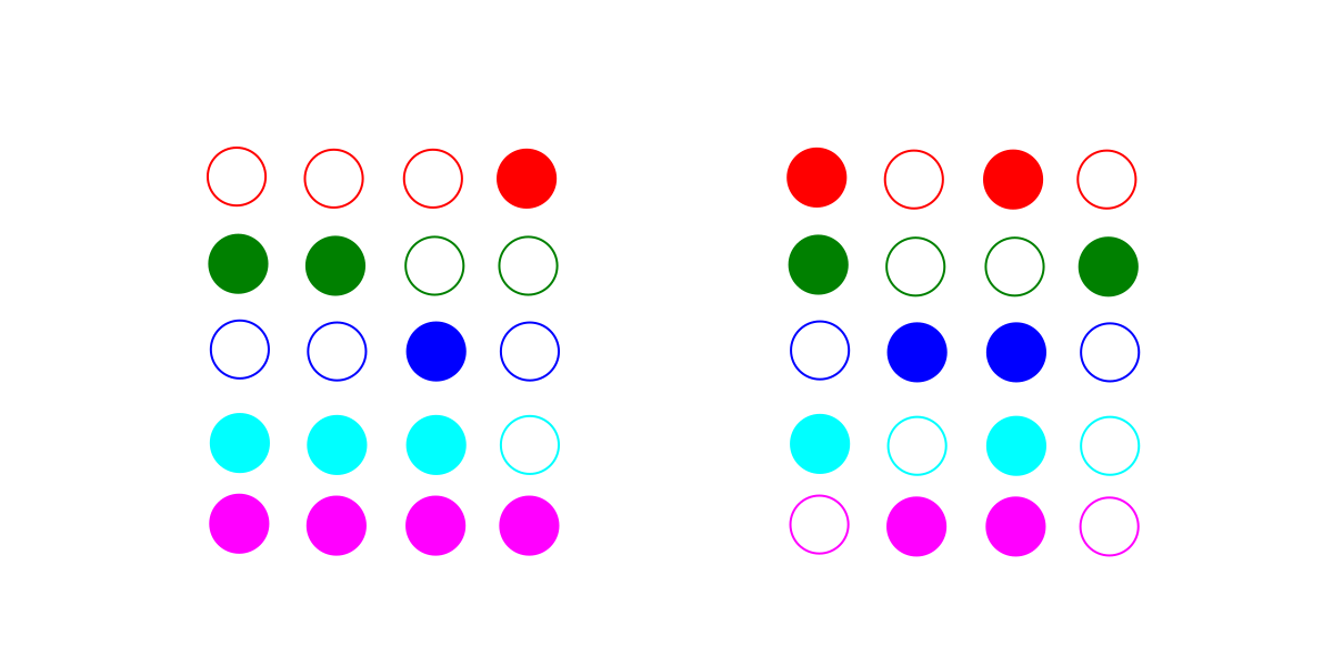
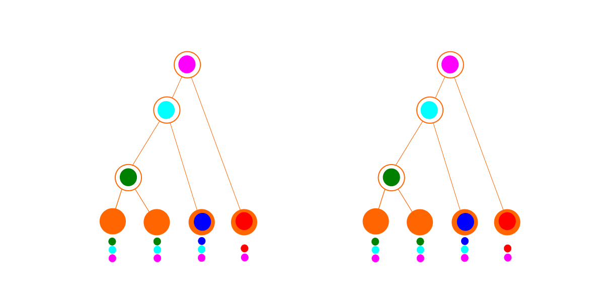
The first set of data (on the left above) fits a tree perfectly (below left). The optimal dependency graph (below right) looks identical to the tree, but because of the extra penalties due to being a dependency graph, it loses out: the best explanation for this data is a tree.

For the second set of data, we can still fit a tree (below left), but it is a mess. We have to delete genes so many times to make it fit that the hypothesis becomes quite improbable. In contrast, the dependency graph finding algorithm finds a set of modules with no deletions. As a result, the dependency graph (below right) wins for this data set. In practice, with more complicated data, the best dependency graph may also involve some deletions. (Just because a module is imported doesn’t necessarily mean everything in it is used, and it is also possible for a designed species to have lost genes that it once had.)

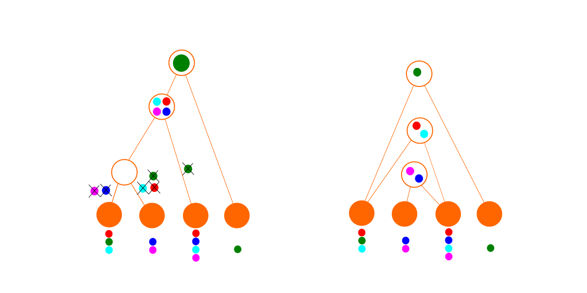
The method does not have to find the best dependency graph, because we know that the best dependency graph is at least as good as the best one we found, and thus the dependency graph is at least that much better than the tree hypothesis. 

Applying the Method

This is how the model selection method works in principle. In the paper, you can see that Ewert tested the method by generating graphs from real software, from various evolutionary simulations, and from random data (a null hypothesis where genes for each species were drawn randomly from a single common pool). He finds that it correctly identifies trees from evolutionary processes (albeit simulated evolution), and correctly identifies dependency graphs from compiled software, and correctly identifies the random data too. 

The really exciting thing is what happens when he looks at biological data. However different biology might be from software, the strange result is that the big picture of biology seems to be objectively much more like software than like evolution. 

One Last Comment

Finally, one reason why I love this paper is it helps explain why Darwin’s tree of life has been accepted by many reasonable people up to now. The reason is: when there isn’t much data, the simpler model wins by default. But now that we have more biological data than ever before, and now that our own understanding of design/engineering/technology has increased in ways that Darwin never could have imagined, we can begin to be able to see that a slightly more complex model could be a much more powerful explanation.  

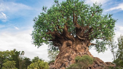
Photo: Tree of Life, at Walt Disney World Resort, by KirkMoorePhoto [CC BY-SA 4.0 ], from Wikimedia Commons.